14 Linear Algebra

A large number of problems in physics can be formulated in the language of linear algebra. Not only is quantum mechanics "just" linear algebra over a complex vector space but we encounter repeatedly the case that a large number of equations have to be solved simultaneously in a form that makes them amenable to linear algebra methods.

Basic problems in linear algebra

Coupled linear equations

Given a known \(N \times N\) matrix \(\mathsf{A}\) and an \(N\)-element vector \(\mathbf{b}\), the matrix equation

\begin{gather} \mathsf{A} \mathbf{x} = \mathbf{b} \end{gather}

represents a system of \(N\) coupled linear equations in the \(N\) unknowns \(\mathbf{x} = (x_1, x_2, \dots, x_N)\).

Eigenvalue problem

The matrix equation

\begin{gather} \mathsf{A} \mathbf{x}_i = \lambda_i \mathbf{x}_i \end{gather}

is the eigenvalue problem and a solution provides the eigenvalues \(\lambda_i\) and corresponding eigenvectors \(\mathbf{x}_i\) that satisfy the equation.

Matrix inverse

Sometimes you want to explicitly find the inverse of a matrix, \(\mathsf{A}^{-1}\),

\begin{gather} \mathsf{A} \mathsf{A}^{-1} = \mathsf{A}^{-1} \mathsf{A} = \mathsf{1} \end{gather}

If the matrix is singular (i.e., the inverse does not exist or equivalently, \(\det\mathsf{A} = 0\)) one can still obtain a useful equivalent of the inverse, \(\mathsf{W}^{-1}\), through singular value decomposition ("SVD")

\begin{gather} \mathsf{A} = \mathsf{U} \mathsf{W} \mathsf{V}^{T} \end{gather}

where \(\mathsf{W} = \mathrm{diag}(w_j), \ 1 \leq j \leq N,\) is a diagonal matrix and the other matrices are orthogonal \(\mathsf{U}\mathsf{U}^{T} = \mathsf{V} \mathsf{V}^{T} = \mathsf{1}\)).¹ For non-singular matrices

\begin{gather} \mathsf{A}^{-1} = \mathsf{V}\, \mathrm{diag}\left(\frac{1}{w_j}\right) \, \mathsf{U}^{T} \end{gather}

but even for singular matrices

\begin{gather} \mathbf{x} = \mathsf{V} \mathsf{W}^{-1} \mathsf{U}^{T}\, \mathbf{b} \end{gather}

will be a useful answer:

• For a \(N \times N\) matrix, values \(w_j = 0\) indicate precisely where \(\mathsf{A}\) is singular and very small \(w_j\) also alert you to possible numerical problems (the solution might easily become dominated by round-off error and the matrix is said to be "ill-conditioned").
• For an overdetermined system (more equations than unknowns²) \(\mathbf{x}\) solves the least-squares fitting problem and determines the solution that minimizes the deviation in the least-squares sense.
• For an underdetermined system (fewer equations than unknowns³) it can be used to find all the vectors that span the solution space.

Numerical solution

Efficient algorithms exist to solve these problems and we will primarily use the optimized algorithms in the numpy.linalg package:

import numpy.linalg

For most linear algebra work you should be using double precision because diagonalization routines and eigenvalue solvers have problems with nearly singular matrices and the better the machine precision is, the better one can distinguish a nearly singular matrix from a truly singular one.

Problem: One rod, two masses, three strings

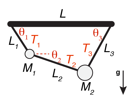
Following Computational Physics (Chapter 6), we want to solve the problem of two masses suspended via three strings from a horizontal rod. The problem with a single mass is trivial and fully determined by the geometry. The problem with two masses is hard but by formulating it as a system of nine coupled non-linear equations in nine unknowns (the three tensions \(T_i\) and, for convenience, we treat \(\sin\theta_i\) and \(\cos\theta_i\) as independent)

\begin{gather} \mathbf{f}(\mathbf{x}) = \mathbf{0} \end{gather}

we can use the generalization of the Newton-Raphson algorithm to \(n\) dimensions to solve it. The generalization involves the computation of the "\(n\)-dimensional derivative", the Jacobian matrix \(J_{ij} = \frac{\partial f_i}{\partial x_j}\), and the Newton-Raphson method becomes to repeatedly solve the linear matrix problem

in order to improve the guess for the solution, \(\mathbf{x}\), with

Class material

The Jupyter notebook 14_Linear_Algebra.ipynb contains the (life-coded) lecture notes on basic linear algebra. Skeleton code for in-class exercises can be found in 14_Linear_Algebra-students-1.ipynb.⁴

To get started on the 1 rod/2 masses/3 strings problem work with the notebook 14_String_Problem-Students.ipynb. The full solution can be found in 14_String_Problem.ipynb.

The notebook 14_SVD.ipynb shows the principles and applications of SVD (with skeleton code in 14_SVD-Students-1.ipynb).

Additional resources:

• Computational Physics: Chapter 6
• 14_linear_algebra notebook (PDF)
• Lecture notes for the 1 rod/2 masses/3 strings problem (PDF) and solution for the problem (PDF)
• 14_SVD notebook (PDF)
• Numerical Recipes in C, WH Press, SA Teukolsky, WT Vetterling, BP Flannery. 2nd ed, 2002. Cambridge University Press. Chapter 2.

Footnotes