06 Stochastic Dynamics with NumPy

23 Feb 2021

Stochastic dynamics or Brownian dynamics describe the movement of particles under friction and random collisions with other particles. A typical example is the random motion of small particle in a bath of solvent molecules.

We will use numpy to generate the random collisions and simulate stochastic particle movements.

Langevin dynamics

Stochastic dynamics is governed by the overdamped Langevin equation (in 1D) (see Resources for background reading):

\begin{equation} \frac{dx}{dt} = \frac{1}{m\gamma}(f + f_\text{random}) \end{equation}

where \(\gamma\) is the friction coefficient, \(f(x) = -dU(x)/dx\) the deterministic force (derived from a potential \(U(x)\), and \(f_\text{random}\) is a random force, which accounts for the random kicks of solvent molecules.

We discretize the equation for small time steps \(\Delta t\) (via \(dx/dt \approx \Delta x/\Delta t\))

\begin{equation} \Delta x = \frac{\Delta t}{m\gamma}(f + f_\text{random}) = \Delta x_\text{deterministic} + \Delta x_\text{random} \end{equation}

so that we can simulate the particle movement and obtain the trajectory \(x(t)\) in discrete steps \(x_j = x(j \Delta t)\):

\[ x_{j+1} = x_j + \Delta x = x_0 + \sum_{k=1}^j \Delta x \]

where \(\Delta x\) has to have been calculated for every step.

To account for the right size for the fluctuations, the random force must be uncorrelated Gaussian noise with zero mean and variance \(\sigma^2 = \frac{2 k_B T \Delta t}{m \gamma}\).

Simple diffusion

If there is no deterministic force present then the particle diffuses randomly,

\begin{equation} \Delta x = \Delta x_\text{random}. \end{equation}

Using the above equation, we can simulate the stochastic trajectory of a randomly diffusing particle.

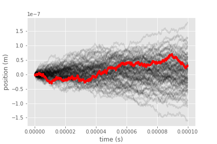Diffusion trajectories. The 1D random movement of a Brome Mosaic Virus in water was simulated for 10,000 time steps and repeated 100 times. A single realization of the stochastic diffusion trajectory is highlighted in red.

Analysis of the trajectory ensemble shows that on average the mean squared distance (MSD) relative to the starting point increases linearly with time,

\begin{equation} \lim_{t\rightarrow+\infty} \langle(x(t) - x_0)^2\rangle = 2 D t \end{equation}

where the constant of proportionality is two times the diffusion coefficient \(D\).

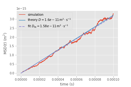Mean square displacement (1D) as function of time for diffusion. The MSD of the simulation trajectories (red) increases linear with time as predicted by theory (blue line). A fit of \(y = 2Dt\) to the simulation data recovers the true diffusion coefficient almost perfectly (purple dashed line).

Random walk on a lattice (optional)

A random walk is a mathematical object, known as a stochastic or random process, that describes a path that consists of a succession of random steps on some mathematical space such as the integers or real numbers (as in the Langevin example above).

A popular random walk model is that of a random walk on a regular lattice, where at each step the location jumps to another site according to some probability distribution. In a simple random walk, the location can only jump to neighboring sites of the lattice, forming a lattice path. In simple symmetric random walk on a locally finite lattice, the probabilities of the location jumping to each one of its immediate neighbors are the same.¹

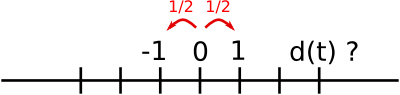Simple 1D random walk. At every time step, a particle can hop to the left or right with equal probability. How far from the origin will it have moved after time t, expressed as the distance \(d(t)\)? Image Source: SciPy Lectures 1.3.2 NumPy: Numerical operations on arrays: Reductions by Emmanuelle Gouillart, Didrik Pinte, Gaël Varoquaux, and Pauli Virtanen.

The random walk also leads to a diffusion process with an equivalent diffusion coefficient if one associates an average time with each jump.

Implementing the random walk on a lattice is a good exercise in using numpy.

Class material

The class will be presented in a Jupyter notebook, 06-stochastic_dynamics.ipynb.

You can load the notebook yourself. Update your local PHY494-resources repository²

Resources

• NumPy Quickstart Tutorial
• SciPy Lectures 1.3.2 NumPy: Numerical operations on arrays: Reductions by Emmanuelle Gouillart, Didrik Pinte, Gaël Varoquaux, and Pauli Virtanen.
• Daniel M Zuckerman. Physical Lens on the Cell Diffusion FAQ: The basics
• Daniel M Zuckerman. Physical Lens on the Cell Advanced Diffusion: Probability Distributions and the Fokker-Planck/Smoluchowski Equation
• Daniel M Zuckerman, Statistical physics of biomolecules: An introduction. CRC Press, Boca Raton, FL, 2010.
• Udo Seifert, Stochastic thermodynamics, fluctuation theorems and molecular machines. Reports on Progress in Physics, 75 (2012), 126001.

---

Footnotes